MthSc 106 Laboratory

Linearization and Newton's Method

Instructions

You are to read through this Maple worksheet and perform any tasks found within the laboratory. Please answer the questions presented with descriptive complete sentences . You are encouraged to work in groups, but each person will need to turn in their own "lab report." The lab report must be word processed. You may use Maple or any other software (such as Word or Scientific WorkPlace) to produce your lab report. The lab report is due one week from today. If you have any questions, do not hesitate to ask. Enjoy and have fun!

Please evaluate any execution cells in the Initialization cell below.

Initialization

> TangentPlot:=proc(expr,r1::name=range,c::realcons)

> local x,a,b,f,g,m,ptplot,pict;

> with(plots);

> with(plottools):

> x:=lhs(r1);

> a:=lhs(rhs(r1));

> b:=rhs(rhs(r1));

> f:=unapply(expr,x);

> m:=subs(x=c,diff(f(x),x));

> g:=unapply(m*(x-c)+f(c),x);

> ### WARNING: the definition of the type `symbol` has changed'; see help page for details
ptplot:=plot([[c,f(c)]],style=point,symbol=circle,color=black);

> pict:=plot([f(x),g(x)],r1,color=[blue,red]);

> display([pict,ptplot]);

> end:

> TangentSlope:=proc(expr,r1::name=realcons)

> local x,a,f,m;

> x:=lhs(r1);

> a:=rhs(r1);

> f:=unapply(expr,x);

> m:=subs(x=a,diff(f(x),x));

> m;

> end:

> NewtonsMethodTable:=proc(expr,r1::name=realcons,r2::name=posint)

> local x,f,a,n,N,g,y,newtab,i;

> x:=lhs(r1);

> f:=unapply(expr,x);

> a:=rhs(r1);

> n:=lhs(r2);

> N:=rhs(r2);

> g:=unapply(diff(f(x),x),x);y[1]:=evalf(a);

> for i from 2 to N do

> y[i]:=evalf(y[i-1]-f(y[i-1])/g(y[i-1]));

> od;

> newtab:=matrix([[`n`,` `, `|`,` `, `x[n]`],

> [`_____`,` `,`|`,` `,`__________`],

> seq([i,` `,`|`,` `,y[i]],i=1..N)])

> end:

> NewtonsMethodPlot:=proc(expr,startpt::name=realcons,num::name=posint)

> local x,a,n,N,f,g,p,i,points,pict1,pict2,pict3,ptlist,

> xmin,xmax,dist,points1,points2,j,linepicts,

> picts,ptplots,fpicts,ptplot;

> with(plots);

> with(plottools);

> x:=lhs(startpt);

> a:=evalf(rhs(startpt));

> n:=lhs(num);

> N:=rhs(num);

> if N<2 then

> ERROR(`You must have at least 2 iterates,

> i.e., n must be greater than 1.`);

> else

> f:=unapply(expr,x);

> g:=unapply(diff(f(x),x),x);

> p[1]:=evalf(a);

> for i from 2 to N do

> p[i]:=evalf(p[i-1]-f(p[i-1])/g(p[i-1]));

> od;

> points1:=[seq([p[i],0],i=1..N)];

> points2:=[seq([p[i],f(p[i])],i=1..N)];

> xmin:=min(seq(p[i],i=1..N));

> xmax:=max(seq(p[i],i=1..N));

> dist:=xmax-xmin;

> pict1:=plot(f(x),x=xmin-(.1)*dist..xmax+(.1)*dist,

> color=blue);

> for i to N do

> points[2*i-2]:=points1[i];

> points[2*i-1]:=points2[i];

> od;

> linepicts:=seq(plot([seq(points[i],i=0..j)],

> x=xmin-(.1)*dist..xmax+(.1)*dist,

> style=line,linestyle=2,color=violet),

> j=1..2*N-1);

> picts:=seq(display([pict1,linepicts[i]]),

> i=1..2*N-1);

> ptplot[1]:=PLOT(POINTS([p[1],0],SYMBOL(CIRCLE),COLOUR(RGB,1,0,0)));

> for j from 2 to N do

> ptplot[j]:=plot([[points1[j]],

> [seq(points1[i],i=1..j-1)]],style=point,

> ### WARNING: the definition of the type `symbol` has changed'; see help page for details
symbol=circle,color=[red,navy]);

> od;

> ptplots:=seq(display([pict1,ptplot[i]]),i=1..N);

> fpicts[0]:=PLOT(POINTS([p[1],0],SYMBOL(CIRCLE),COLOUR(RGB,1,0,0)));

> for i to N-1 do

> fpicts[3*i-2]:=display(

> [ptplots[i],fpicts[3*i-3]]);

> fpicts[3*i-1]:=display(

> [picts[2*i-1],fpicts[3*i-2]]);

> fpicts[3*i]:=display([picts[2*i],fpicts[3*i-1]]);

> od;

> fpicts[3*N-2]:=display([ptplots[N],fpicts[3*N-3]]);

> display([seq(fpicts[i],i=1..3*N-2)],

> insequence=true);

> fi;

> end:

> fn1:=unapply(piecewise(x>=2,sqrt(x-2),-sqrt(2-x)),x):

> fn2:=unapply(piecewise(x>=4,sqrt(x-4),sqrt(4-x)),x):

>

Overview

Many times we are faced with situations which force us to work with very complicated (a.k.a.ugly) functions. In many cases we can replace these "messy" functions with approximations which are easier to work with. For the most part, the simplicity of the approximation depends on the nature of the function and the accuracy we need to achieve. The simpliest type of approximation to a differentiable function near a point ( ) is a linear approximation called the linearization of f at
.

In this lab we will discover which linear function makes up the linearization of a differentiable function f at . And after we get our linearizations straight, we will see how linear approximations to a function can be used to create an iterative process (called Newton's Method ) which can determine solutions to the equation .

Linear approximations to a differentiable function

Some functions can be hard to work with computationally. Who wouldn't cringe at the task of computing functional values for the function

,

or for that matter, finding roots of this function without the aid of a computer or calculator ? Horrors! Of course in this age of technology we wouldn't have to worry too much about a problem such as this. Even so, depending on the types of computations and the required accuracy of the computations, it is sometimes to our advantage to replace the complicated function f with an approximation which is easier to handle computationally. Certainly there are many ways in which to approximate a function. We will concentrate on the simpliest substitute for a function: a linear function.

The idea of replacing an arbitrary differentiable function with a linear function should set off all kinds of warning bells. After all, if a differentiable function is not linear, it's graph probably has some "curve" or "curves" in it, and so, doesn't resemble a line. Right? Globally this is certainly the case, but the difference between a nonlinear curve and a line is not so easily seen if we restrict our attention to a small portion of the graph. To illustrate this, let's examine the function

.

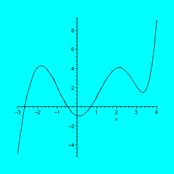
We begin by obtaining a sketch of the graph of f on the interval . Please evaluate the execution cell below.

> plot(7/360*x^6+1/120*x^5-37/72*x^4+1/8*x^3+539/180*x^2-19/30*x-1,

> x=-3..4,color=blue);

>

As you can see by the sketch, the function doesn't appear to be anything close to linear. Thus we conclude the function's "global" behavior is not linear. But what about the function's "local" behavior? To get a good understanding of the local nature of a differentiable function, we begin by focusing our attention on a few of the "local hot spots!"

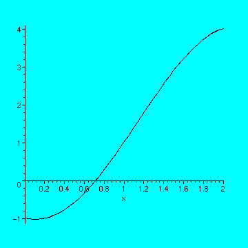
Let's start by examining the behavior of f near . It might be helpful if we look at a picture of f which zooms in towards . Please evaluate the cell below.

> plot(7/360*x^6+1/120*x^5-37/72*x^4+1/8*x^3+539/180*x^2-19/30*x-1,

> x=0..2,color=blue);

>

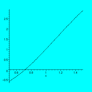
The function is still not linear over this interval, but it now seems plausible to use a linear approximation for f on this interval. Perhaps we should narrow our focus further. Please evaluate the cell below.

> plot(7/360*x^6+1/120*x^5-37/72*x^4+1/8*x^3+539/180*x^2-19/30*x-1,

> x=.5..1.5,color=blue);

>

1. Does the function appear to be more or less linear on this interval? Justify your answer.

2. Find an interval about for which the graph of the function f appears to be linear. Paste a copy of the sketch in your lab report.

3. Find an interval about for which the graph of the function f appears to be linear. Paste a copy of the sketch in your lab report.

At this point we are probably convinced that "small chunks" of f do appear linear. So it makes sense to approximate f locally by a linear function. Now for the next question: if we want to use a linear function to approximate f near , what linear function do we use? Hmm. If our linear approximation is to be accurate near , we would want the linear function to agree with the function at , and we would want the line to have the same "slope" as the function at . Let's translate our "wish list" into a set of conditions. Let represent the linear function which is the linear approximation to f near . So our conditions become:

1. .

2. f '( ), where m is the slope of the linear function L.

Thus the linear approximation of f near is a line with slope f '( a ) going through the point ( ) . This linear approximation is called the linearization of f near .

4. Find the formula for for a differentiable function f near (i.e., find the linear function with slope f '(a) and ). What familar line is this?

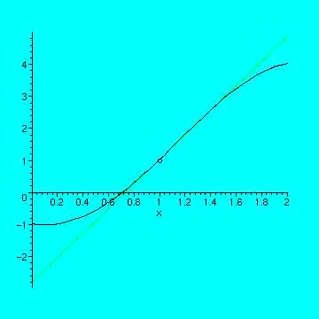
So we see the linear approximation to use to approximate a differentiable function near is just the tangent line to the curve of f at . It would be nice to have some visual justification. We can get it by sketching the graph of f and the tangent line to f at on the same coordinate plane. This is easily achieved by the (local) Maple command TangentPlot . A template for TangentPlot is given below:

TangentPlot(f(x),x=a..b,c);

sketches the graphs of (in blue) and the tangent line to f at (in red) on the interval .

To obtain a graph of the function and it's tangent line at on the interval , we need only to evaluate the cell below.

> TangentPlot(7/360*x^6+1/120*x^5-37/72*x^4+1/8*x^3+539/180*x^2-19/30*x-1,

> x=0..2,1);

>

We see the tangent line is a pretty good approximation to the curve from about 0.8 to 1.5, but it loses it's accuracy elsewhere in the interval.

5. Use TangentPlot to find an interval about for which the graphs of the function f and the tangent line to f at appear to coincide. Paste a copy of the sketch in your lab report.

When we use a linear approximation for f near , we are replacing the -value with the -value, i.e., we are saying

» .

Isn't this amazing? We can approximate a very nasty looking function with a function of the form ! While this is a wonderful result, we must remember nothing comes for free: this approximation is only good when we are "very close" to the point of tangency. And the meaning of "very close" changes with the function and the portion of the function we are interested in.

Let's see how to use this approximation. If we wanted to use a linear approximation to estimate , where f is given by

,

we would use the tangent line to the graph of f at . (Why use ?) So our first step is to determine the function . The (local) Maple command TangentSlope can help facilitate this step. A template for TangentSlope is given below.

TangentSlope(f(x),x=a);

computes f '(a).

Please evaluate the cell below to compute f '(1) .

> TangentSlope(7/360*x^6+1/120*x^5-37/72*x^4+1/8*x^3+539/180*x^2-19/30*x-1,x=1);

>

Next we need to find the point on the line of tangency. The x -coordinate of the point is 1 and the y -coordinate is f(1) . Please evaluate the cell below to compute f(1) .

> subs(x=1,7/360*x^6+1/120*x^5-37/72*x^4+1/8*x^3+539/180*x^2-19/30*x-1);

>

Thus the linearization is

f '(1) .

Our last step is to compute . Please evaluate the cell below.

> subs(x=1.05,23/6*(x-1)+1);

>

Hence the linear approximation to is 1.19166667. How good is the approximation? Evaluate the cell below to find the actual value of .

> subs(x=1.05,7/360*x^6+1/120*x^5-37/72*x^4+1/8*x^3+539/180*x^2-19/30*x-1);

>

6. Use a linear approximation to the function to obtain an approximation to . Be sure to include the linearization you used to get your estimate in your lab report. How accurate is your approximation?

Newton's Method

Ever wonder how the SOLVE button on a calculator or the solve command in Maple is able to find solutions (or at least approximations to solutions) so "effortlessly" to many equations? Obviously the calculator and the Maple command run through a program which finds solutions. But how do the programs do this? The answer is beyond the scope of this course, but we can examine one iterative process which is just a portion of the programming used in most solver programs. The process uses linearizations of a differentiable function to find roots of a function (i.e., solutions to the equation ). The name of this procedure is Newton's Method .

Let's consider the function . First we'll ask Maple to find the roots of this function using the solve command. Please evaluate the cell below.

> solve(cos(x)-x^2=0,x);

>

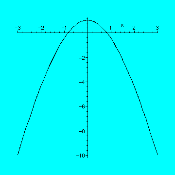
What happened? Absolutely nothing! Are there any solutions? We will next graph the function to see if it has any (real) roots (i.e., -intercepts). Please evaluate the cell below.

> plot(cos(x)-x^2,x=-3..3,color=blue);

>

Its pretty clear from the picture the function has two real roots. Why didn't Maple find them? The solve command sometimes needs help. But that is not what we're here to do. Instead we will explore a method which will allow us to (in many cases) compute approximations to the roots.

We begin by trying to find the root near . Since we've had no luck with the function, let's use the linearization of f at to get an approximation to the root. (Why? Its easy to find the -intercept of a line.) So we need to compute the -intercept of the line

f '(1) or .

Please execute the cell below to find the -intercept of the linearization.

> solve(-2.841470985*x+2.381773291=0,x);

>

So our first approximation to the root is .8382184100. The figure below illustrates how we obtained our first estimate.

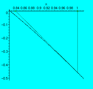
Let's recap what has happened so far. Our first step was to make a guess near the actual root. We began with . Next we found the linearization of f near x = 1 . Then we found the -intercept of the linearization. This gave us our second estimate of the root near 1. As we can see from the figure above, our second approximation is much closer than the first "guess." How do we get closer to the root? Why not repeat the same procedure as above, but now using the linearization of f at .

7. Find the linearization of f at . Then use solve to find the x -intercept of the line and hence our next approximation to the root of the function f near .

As you can see, the above process can be repeated as many times as you like, with the -th term (i.e., ) given by

.

These calculations can become tedious. The (local) Maple command NewtonsMethodTable can perform these calculations for us. A template for NewtonsMethodTable is given below:

NewtonsMethodTable(f(x),x=a,n=N);

produces a table with the first N terms in the Newton's Method iterative process beginning with .

Please evaluate the cell below to obtain the first 10 terms with .

> NewtonsMethodTable(cos(x)-x^2,x=1,n=10);

>

Notice the terms from on are all the same value. Before we make any conclusions, let's get a picture of what is happening. The (local) Maple command NewtonsMethodPlot can provide such a picture. A template for NewtonsMethodPlot is given below:

NewtonsMethodPlot(f(x),x=1,n=N);

provides an animation which depicts the Newton's Method process through the first N terms.

Please execute and then animate the cell below.

> NewtonsMethodPlot(cos(x)-x^2,x=1,n=10);