Go to:Table of Contents

Differential Entropy and Probability Distributions

Probability distributions plays a key role in statistical analysis. This is because standard theoretical distributions are indeed the statistical models for different kinds of situations. For example, consider a random experiment, the outcome of which can be classified one of two mutually exclusive and exhaustive ways, say, success or failure. Then if the experiment is repeated n times, the binomial distribution is the model in determining the probability of number of successes. The Poisson distribution may serve as an excellent mathematical model in a number of situations. The number of road accidents in some unit of time, the number of insurance claims in some unit of time, the number of telephone calls at a swichtboard in some unit of time etc.. are all governed by the Poisson model.

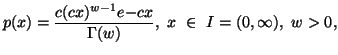
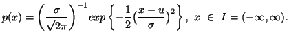
An another example, the gamma distribution is frequently used as the probability model for waiting times; for instance, in testing bulbs until they fail, then if the random variable $X$ is the time needed to obtain exactly $k$ failures, where $k$ is a fixed positive integer, the distribution of $X$ is the gamma distribution. Perhaps, the most used distribution in statistical analysis is the normal distribution. It is encountered in many different situations, e.g., the score on a test, the length of a newly born child, the yield of a grain on a plot of ground, etc.. The normal distribution can also be used as an approximation to many other distribution, e.g., Poisson distribution, Bionomial distribution etc..

In this subsection, we use maximum entropy principle to characterize important probability distributions. This provides not only a new way of characterizing them but also brings out an important underlying unity in these distributions (ref. Gokhale, 1975 [40], Kagan et al., 1973 [53], Kapur, 1989 [60];1992 [62]).

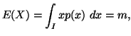
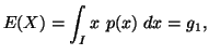
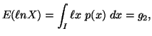
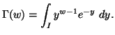
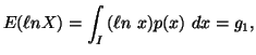
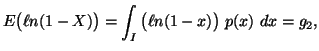
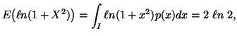
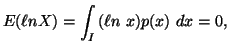
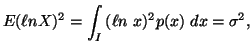
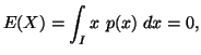
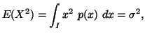
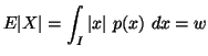
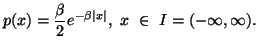
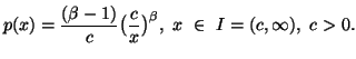
In the following property we characterize via entropy maximum principle various probability distributions subject to the constraint $\int_{I}{p(x)\ dx}=1$, $p(x)\geq 0$,$x\ \in\ I$ along with others, where the interval I vary accordingly.

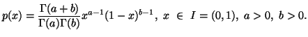
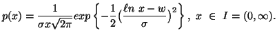
Property 1.76. We have

(i) The probability distribution $p(x)$ maximizing the differential entropy (1.13) is the uniform distribution given by 

$$p(x)={1\overb-a},\ x\ \in\ I=(0,1).$$

(ii) The probability distribution $p(x)$ maximizing the differential entropy (1.13) subject to the constraint 

$$E(X)=\int_{I}{x p(x)\dx} = m,$$ is the exponential distribution given by $$p(x)=w\ exp(-wx),\ x\ \in I=(0,\infty),\ w>0.$$

(iii) The probability distribution $p(x)$ maximizing the differential entropy (1.13) subject to the constraints 

$$E(X)=\int_{I}{x\ p(x)\dx} = g_1,$$ and  $$E(\ell nX)=\int_{I}{\ell x\ p(x)\ dx} = g_2,$$ is the gamma distribution given by $$p(x)={c(cx)^{w-1}e{-cx}\over \Gamma (w)},\ x\ \in\I=(0,\infty),\ w>0,$$ where  $$\Gamma (w)=\int_{I}{y^{w-1}e^{-y}\dy}.$$

(iv) The probability distribution $p(x)$ maximizing the differential entropy (1.13) subject to the constraints 

$$E(\ellnX)=\int_{I}{(\ell n\ x) p(x)\ dx} = g_1,$$ and  $$E\big(\elln(1-X)\big)=\int_{I}{\big(\ell n(1-x)\big)\ p(x)\ dx} = g_2,$$ is the beta distribution given by  $$p(x)={\Gamma(a+b)\over\Gamma(a)\Gamma(b)}x^{a-1}(1-x)^{b-1},\ x\ \in \ I=(0,1),\ a>0,\b>0.$$

(v) The probability distribution $p(x)$ maximizing the differential entropy (1.13) subject to the constraint 

$$E\big(\elln(1+X^2)\big)=\int_{I}{\ell n(1+x^2)p(x)dx}=2\ \ell n\ 2,$$ is the Cauchy distribution given by  $$p(x)={1\over \pi (1+x^2)}, \x \ \in\ I=(-\infty, \infty).$$

(vi) The probability distribution $p(x)$ maximizing the differential entropy (1.13) subject to the constraints 

$$E(\ellnX)=\int_{I}{(\ell n\ x)p(x)\ dx} =0,$$ and  $$E(\ellnX)^2=\int_{I}{(\ell n\ x)^2p(x)\ dx} =\sigma^2,$$ is the log-normal distribution given by  $$p(x)={1\over \sigmax\sqrt{2\pi}}exp \left\{-{1\over 2}\big( {\ell n\ x-w\over\sigma}\big)^2\right\},\ x\ \in\ I=(0,\infty).$$

(vii) The probability distribution $p(x)$ maximizing the differential entropy (1.13) subject to the constraints 

$$E(X)=\int_{I}{x\ p(x)\dx} =0,$$ and  $$E(X^2)=\int_{I}{x^2\ p(x)\ dx} =\sigma^2,$$ is the normal distribution given by  $$p(x)=\bigg({\sigma\over\sqrt{2\pi}}\biggr)^{-1}exp \left\{-{1\over 2}\big( { x-u\over\sigma}\big)^2\right\},\ x \ \in\ I=(-\infty, \infty).$$

(viii) The probability distribution $p(x)$ maximizing the differential entropy (1.13) subject to the constraint 

$$E\vert X\vert=\int_{I}{\vert x\vert\p(x)\ dx}=w$$ is the Laplace distribution given by $$p(x)={\beta\over 2}e^{-\beta\vert x\vert},\ x\ \in \I=(-\infty,\infty).$$

(ix) The probability distribution $p(x)$ maximizing the differential entropy (1.13) subject to the constraint 

$$\int_{I}{\ell n\ x\dx}=m,$$ is the Pareto distribution given by $$p(x)={(\beta-1)\over c}\big({c\over x}\big)^{\beta},\ x\ \in\I=(c,\infty),\ c>0.$$